CS M146 Midterm Cheatsheet
#Computers
Misc
- $\displaystyle \lVert \vec{x}\rVert_{p}=\left( \sum_{i}\lvert x_{i}\rvert^{p} \right)^{\frac{1}{p}}$
- $\displaystyle L_{\text{ridge}}=\lambda \lVert \theta\rVert_{2}$, circular
- $\displaystyle \nabla b^{^{\top}}x=b$
- $\displaystyle \nabla x^{T}Ax=2Ax$
Validation
$\displaystyle CV(\text{Model})=\frac{1}{K}\sum_{i = 1}^{K}L(\hat{f}{C{-i}}(C_{i}))$
- $\displaystyle K=$ number of chunks
- $\displaystyle \hat{f}{C{-i}}=$ model fitted to the training set of all chunks that aren't $\displaystyle C_{i}$, the validation set
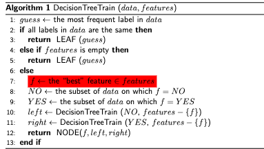
Decision Trees
- $\displaystyle \Delta H=H_{\text{parent}}-\sum_{i}p_{i}H_{\text{children}}$
- $\displaystyle H(X)\equiv -\mathbb{E}[\log p(X)]$
- $\displaystyle g=1-\sum_{i}p_{i}^{2}$
K-Nearest Neighbors
$\displaystyle \text{nn}{k}(x)=\text{argmin}{n\in \left( [N]-\sum_{i = 1}^{k-1}\text{nn}{i}(x) \right)}\lVert x-x{n}\rVert^{2}_{2}$
- Gives the index in $\displaystyle [N]$ of the $\displaystyle k$th nearest neighbor of $\displaystyle x$, or the data point we're interested in classifying
- $\displaystyle [N]$ is an array of indices for each data sample point
- We use the square of the L2 norm here to calculate distance but other measures could work
$\displaystyle \text{knn}(x)=\left{\text{nn}{1}(x),\text{nn}{2}(x),\ldots ,\text{nn}_{K}(x) \right}$
- Gives the set of indices of the $\displaystyle K$ nearest neighbors to $\displaystyle x$
$\displaystyle v_{c}=\sum_{n\in \text{knn}(x)}\mathbb{I}(y_{n}==c)~\forall~c\in [C]$
- Gives the number of "votes" for a particular class/label $\displaystyle c$
- We iterate over each of the $\displaystyle K$-nearest neighbors and increment by one every time the neighbor equals the class of interest
$\displaystyle y=h(x)=\text{argmax}{c\in [C]}v{c}$
- The prediction is the class $\displaystyle c$ that maximizes the number of votes
Steps To Classify
- Initialize
- Place the data point in a feature space
- Calculate Distance
- Find the Euclidean distance from the data point with all other labeled data
- May have to normalize data point values along different coordinates to be Z-scores for each coordinate
- Sort Distance
- Sort distances of the data point with other labeled data points in increasing order
- For classification, the most common class of $\displaystyle k$-nearest neighbors determines the data point class
- For regression, use the average of the $\displaystyle k$-nearest neighbors' labels
Perceptron
- $\displaystyle H=\left{ h|h:\mathbb{X}\rightarrow \mathbb{Y},h(\mathbf{x})=\text{sign}(a) \right}$
$$\displaystyle \text{Margin}(\mathcal{D},w)=\begin{cases}
\text{min}{(x,y)\in \mathcal{D}} \frac{1}{\left\lVert w\right\rVert}y{n}w^{T}x_{n} & \text{for separating hyperplane }w \\-\infty & \text{else}
\end{cases}$$
- $\displaystyle \text{Margin}(\mathcal{D})=\text{max}_{w}\text{Margin}(\mathcal{D},w)$
- $\displaystyle a= \sum_{d = 1}^{D}w_{d}x_{d}+b=w^{T}x+b$
Mistake Bound Theorem
- For a dataset $\displaystyle \left{ (x_{1},y_{1}),\ldots,(x_{N},y_{N}) \right}$ with $\displaystyle R\geq \lVert x_{n}\rVert_{2}$ and labels $\displaystyle y_{n}\in \left{ -1,1 \right}$
- Suppose $\displaystyle ~\exists~u\in \mathbb{R}^{D}:~\exists~\gamma>0\land \gamma\leq y_{n}u^{^{\top}}x_{n}$
- $\displaystyle u$ can be thought of as a $\displaystyle w$ of a candidate for the margin of the dataset
- Then the PerceptronTrainingAlgorithm will make $\displaystyle \leq \frac{R^{2}}{\gamma ^{2}}$ mistakes on the training sequence
- Proof Preliminaries: $\displaystyle w_{0}=0,\left\lVert x_{n}\right\rVert\leq R,y_{n}u^{T}x_{n}\geq \gamma$
- Proof (1/3): After $\displaystyle t$ mistakes, $\displaystyle u^{T}w_{t}\geq t\gamma$ by induction from $\displaystyle w_{0}=0$ and using $\displaystyle u^{T}w_{t+1}=u^{T}(w_{t}+y_{n}x_{n})$
- Proof (2/3): After $\displaystyle t$ mistakes, $\displaystyle \left\lVert w_{t}\right\rVert^{2}\leq tR^{2}$
- Proof (3/3): $\displaystyle R\sqrt{ t }\geq \left\lVert w_{t}\right\rVert\geq u^{T}w_{t}\geq t\gamma$
Logistic Regression
- $\displaystyle J(\theta)=-\sum_{n}\left{ y_{n}\log h_{\theta}(x_{n})+(1-y_{n})\log[1-h_{\theta}(x_{n})] \right}$
- $\displaystyle h_{\theta}(x)=P(y=1|x;\theta)=\sigma(a)=\frac{1}{1+e^{-a}}$
- $\displaystyle \frac{\partial J(\theta) }{\partial \theta}=\sum_{n}\left{ h_{\theta}(x_{n})-y_{n} \right}x_{n}$
Convexity
- $\displaystyle f(\lambda a+(1-\lambda)b)\leq \lambda f(a)+(1-\lambda)f(b),\lambda \in [0,1]\rightarrow f(x)$ is convex
- $\displaystyle f(x)$ is convex $\displaystyle \rightarrow f''(x)>0~\forall~x$
- $\displaystyle \mathbf{H}_{f}\succeq 0\rightarrow f$ is convex
- $\displaystyle x^{\top}Ax\geq 0\rightarrow A\succeq 0$
- $\mathbf{H}{f}=\nabla {x}^{2}f(x)\in \mathbb{R}^{n\times n}:(\nabla {x}^{2}f(x)){ij}=\partial{x{i},x_{j}}f(x)$
Linear Regression
- $\displaystyle \hat{Y}=\hat{\beta}{1}X+\hat{\beta}{0}+\varepsilon$
- $\displaystyle \varepsilon=\eta\sim \mathcal{N}(0,\sigma ^{2})$
- $\displaystyle J(\boldsymbol{\theta})=\sum_{n}[y_{n}-({\theta}{1}X+{\theta}{0})^{2}]=\left\lVert \boldsymbol{y}-\boldsymbol{X\theta}\right\rVert^{2}_{2}$
- The loss function for simple linear regression
- Minimizing this by varying $\displaystyle {\beta}{0}$/$\displaystyle {\beta}{1}$ or $\displaystyle \boldsymbol{\theta}$ gives the linear model that best fits with the data $\displaystyle \boldsymbol{y}$
- $\displaystyle \boldsymbol{y}$ is the target vector
- $\displaystyle {\theta}{1}= \frac{\sum{i}(x_{i}-\bar{x})(y_{i}-\bar{y})}{\sum_{i}(x_{i}-\bar{x})^{2}}$
- $\displaystyle {\theta}{0}=\bar{y}-{\theta}{1}\bar{x}$
- $\displaystyle \text{MSE}(\beta)=\frac{1}{n}\lVert \mathbf{Y-X}\theta\rVert^{2}$
- $\displaystyle \theta=\underset{\beta}{\text{argmin}}\text{,MSE}(\beta)=(\mathbf{X}^{\top}\mathbf{X})^{-1}\mathbf{X}^{\top}\mathbf{Y}$
- $\displaystyle \sigma ^{2}=\sum \frac{(\hat{f}(x)-y_{i})^{2}}{n}$
Regularized
- $\displaystyle \hat{\theta}=(\mathbf{X^{^{\top}}X+\lambda I})^{-1}\mathbf{X^{^{\top}}y}$
- $\displaystyle \nabla J(\mathbf{w})=2(\mathbf{X^{^{\top}}Xw-X^{^{\top}}y+\lambda w})$
Run Times
| Algorithm | Training Time Complexity | Test Time Complexity |
|---|---|---|
| Decision Tree | $O(n \log(n))$ to $O(n^2)$ (depends on splitting strategy) | $O(\log(n))$ (balanced) or $O(n)$ (unbalanced) |
| K-Nearest Neighbors (KNN) | $O(1)$ (no training, just storing data) | $O(n d)$ (linear search) or $O(\log(n))$ (KD-tree, low dimensions) |
| Perceptron | $O(n d)$ per epoch | $O(d)$ |
| Logistic Regression | $O(n d)$ per iteration (gradient-based) | $O(d)$ |
| Linear Regression (Analytical - Normal Equation) | $O(d^3 + n d^2)$ (matrix inversion) | $O(d)$ |
| Linear Regression (Gradient Descent) | $O(n d k)$ (depends on iterations $k$) | $O(d)$ |
| Full Batch Gradient Descent | $O(n d k)$ | $O(d)$ |
| Stochastic Gradient Descent (SGD) | $O(d k)$ | $O(d)$ |
| Mini-Batch Gradient Descent | $O\left(\frac{n}{b} d k\right)$ (where $b$ is batch size) | $O(d)$ |
| - $n$ = number of training samples | ||
| - $d$ = number of features (dimensions) | ||
| - $k$ = number of iterations in gradient-based methods | ||
| - $b$ = batch size for mini-batch gradient descent |
Algorithms